Nexus User Scripts

Users interact with Nexus by writing a Python script that often resembles an input file. A Nexus user script typically consists of six main sections, as described below:

Nexus imports:

functions unique to Nexus are drawn into the user environment.

Nexus settings:

specify machine information and configure the runtime behavior of Nexus.

Physical system specification:

create a data description of the physical system. Generate a crystal structure or import one from an external data file. Physical system details can be shared among many simulations.

Workflow specification:

describe the simulations to be performed. Link simulations together by their data dependencies to form workflows.

Workflow execution:

pass control to Nexus for active workflow management. Simulation input files are generated, jobs are submitted and monitored, output files are collected and preprocessed for later analysis.

Data analysis:

control returns to the user to extract preprocessed simulation output data for further analysis.

Each of the six input sections is the subject of lengthier discussion: Nexus imports, Nexus settings: global state and user-specific information, Physical system specification, Workflow specification, Workflow execution, and Data analysis. These sections are also illustrated in the abbreviated example script below. For more complete examples and further discussion, please refer to the user walkthroughs in Complete Examples.

Nexus imports

Each script begins with imports from the main Nexus module. Items imported include the interface to provide settings to Nexus, helper functions to make objects representing atomic structures or simulations of particular types (e.g. QMCPACK or VASP), and the interface to provide simulation workflows to Nexus for active management.

The import of all Nexus components is accomplished with the brief “from nexus import *”. Each component can also be imported separately by name, as in the example below.

from nexus import settings                   # Nexus settings function
from nexus import generate_physical_system   # for creating atomic structures
from nexus import generate_pwscf             # for creating PWSCF sim. objects
from nexus import Job                        # for creating job objects
from nexus import run_project                # for active workflow management

This has the advantage of avoided unwanted namespace collisions with user defined variables. The major Nexus components available for import are listed in Table 1.

Table 1 Major Nexus components available for import.

component	description
settings	Alter runtime behavior. Provide machine information.
generate_physical_system	Create atomic structure including electronic information.
generate_structure	Create atomic structure without electronic information.
generate_simulation	Create generic simulation object.
generate_pwscf	Create PWSCF simulation object.
generate_vasp	Create VASP simulation object.
generate_gamess	Create GAMESS simulation object.
generate_qmcpack	Create QMCPACK simulation object.
generate_sqd	Create SQD simulation object.
input_template	Create generic input file object.
multi_input_template	Create generic input file object representing multiple files.
generate_pwscf_input	Create PWSCF input file object.
generate_vasp_input	Create VASP input file object.
generate_gamess_input	Create GAMESS input file object.
generate_qmcpack_input	Create QMCPACK input file object.
generate_sqd_input	Create SQD input file object.
Job	Provide job information for simulation run.
run_project	Initiate active workflow management.
obj	Generic container object. Store inputs for later use.

Nexus settings: global state and user-specific information

Following imports, the next section of a Nexus script is dedicated to providing information regarding the local machine, the location of various files, and the desired runtime behavior. This information is communicated to Nexus through the settings function. To make settings available in your project script, use the following import statement:

from nexus import settings

In most cases, it is sufficient to supply only four pieces of information through the settings function: whether to run all jobs or just create the input files, how often to check jobs for completion, the location of pseudopotential files, and a description of the local machine.

settings(
    generate_only = True,                 # only write input files, do not run
    sleep         = 3,                    # check on jobs every 3 seconds
    pseudo_dir    = './pseudopotentials', # path to PP file collection
    machine       = 'ws8'                 # local machine is an 8 core workstation
    )

A few additional parameters are available in settings to control where runs are performed, where output data is gathered, and whether to print job status information. More detailed information about machines can be provided, such as allocation account numbers, filesystem structure, and where executables are located.

settings(
    status_only   = True,                 # only show job status, do not write or run
    generate_only = True,                 # only write input files, do not run
    sleep         = 3,                    # check on jobs every 3 seconds
    pseudo_dir    = './pseudopotentials', # path to PP file collection
    runs          = '',                   # base path for runs is local directory
    results       = '/home/jtk/results/', # light output data copied elsewhere
    machine       = 'titan',              # Titan supercomputer
    account       = 'ABC123',             # user account number
    )

Physical system specification

After providing settings information, the user often defines the atomic structure to be studied (whether generated or read in). The same structure can be used to form input to various simulations (e.g. DFT and QMC) performed on the same system. The examples below illustrate the main options for structure input.

Read structure from a file

dia16 = generate_physical_system(
    structure = './dia16.POSCAR',  # load a POSCAR file
    C         = 4                  # pseudo-carbon (4 electrons)
    )

Generate structure directly

dia16 = generate_physical_system(
    lattice   = 'cubic',           # cubic lattice
    cell      = 'primitive',       # primitive cell
    centering = 'F',               # face-centered
    constants = 3.57,              # a = 3.57
    units     = 'A',               # Angstrom units
    atoms     = 'C',               # monoatomic C crystal
    basis     = [[0,0,0],          # basis vectors
                 [.25,.25,.25]],   #  in lattice units
    tiling    = (2,2,2),           # tile from 2 to 16 atom cell
    C         = 4                  # pseudo-carbon (4 electrons)
    )

Provide cell, elements, and positions explicitly:

dia16 = generate_physical_system(
    units  = 'A',                      # Angstrom units
    axes   = [[1.785,1.785,0.   ],     # cell axes
              [0.   ,1.785,1.785],
              [1.785,0.   ,1.785]],
    elem   = ['C','C'],                # atom labels
    pos    = [[0.    ,0.    ,0.    ],  # atomic positions
              [0.8925,0.8925,0.8925]],
    tiling = (2,2,2),                  # tile from 2 to 16 atom cell
    kgrid  = (4,4,4),                  # 4 by 4 by 4 k-point grid
    kshift = (0,0,0),                  #  centered at gamma
    C      = 4                         # pseudo-carbon (4 electrons)
    )

In each of these cases, the text “C = 4” refers to the number of electrons in the valence for a particular element. Here a pseudopotential is being used for carbon and so it effectively has four valence electrons. One line like this should be included for each element in the structure.

Workflow specification

The next section in a Nexus user script is the specification of simulation workflows. This stage can be logically decomposed into two sub-stages: (1) specifying inputs to each simulation individually, and (2) specifying the data dependencies between simulations.

Generating simulation objects

Simulation objects are created through calls to “generate_xxxxxx” functions, where “xxxxxx” represents the name of a particular simulation code, such as pwscf, vasp, or qmcpack. Each generate function shares certain inputs, such as the path where the simulation will be performed, computational resources required by the simulation job, an identifier to differentiate between simulations (must be unique only for simulations occurring in the same directory), and the atomic/electronic structure to simulate:

relax = generate_pwscf(
    identifier   = 'relax',                   # identifier for the run
    path         = 'diamond/relax',           # perform run at this location
    job          = Job(cores=16,app='pw.x'),  # run on 16 cores using pw.x executable
    system       = dia16,                     # 16 atom diamond cell made earlier
    pseudos      = ['C.BFD.upf'],             # pseudopotential file
    files        = [],                        # any other files to be copied in
    ...                                       # PWSCF-specific inputs follow
    )

The simulation objects created in this way are just data. They represent requests for particular simulations to be carried out at a later time. No simulation runs are actually performed during the creation of these objects. A basic example of generation input for each of the four major codes currently supported by Nexus is given below.

Quantum ESPRESSO (PWSCF) generation:

scf = generate_pwscf(
    identifier   = 'scf',
    path         = 'diamond/scf',
    job          = scf_job,
    system       = dia16,
    pseudos      = ['C.BFD.upf'],
    input_type   = 'generic',
    calculation  = 'scf',
    input_dft    = 'lda',
    ecutwfc      = 75,
    conv_thr     = 1e-7,
    kgrid        = (2,2,2),
    kshift       = (0,0,0),
    )

The keywords calculation, input_dft, ecutwfc, and conv_thr will be familiar to the casual user of Quantum ESPRESSO’s PWSCF/pw.x program. Any input keyword that normally appears as part of a namelist in PWSCF input can be directly supplied here. The generate_pwscf function, like most of the others, actually takes an arbitrary number of keyword arguments. These are later screened against known inputs to PWSCF to avoid errors. The kgrid and kshift inputs inform the KPOINTS card in the PWSCF input file, overriding any similar information provided in generate_physical_system.

Note on DFT+U support in Quantum ESPRESSO and Nexus: a new set of keywords was adopted for DFT+U-based methods starting with v7.1 of Quantum ESPRESSO. Both the current (“new”) and old formats are supported by Nexus, but via different keywords.

For v7.1 and above use:

hubbard          = {'U':{'Fe-3d': 5.5}},
hubbard_proj     = 'ortho-atomic',

For older versions use:

U_projection_type = 'ortho-atomic',
hubbard_u        = obj(Fe=5.5),

Examples of this usage can be found in nexus/nexus/examples, e.g., nexus/nexus/examples/qmcpack/rsqmc_quantum_espresso/04_iron_dft_dmc_gcta/iron_ldaU_dmc_gcta.py shows how to run DFT+U calculations for grand-canonical twist averaging using the latest format.

VASP generation:

relax = generate_vasp(
    identifier   = 'relax',
    path         = 'diamond/relax',
    job          = relax_job,
    system       = dia16,
    pseudos      = ['C.POTCAR'],
    input_type   = 'generic',
    istart       = 0,
    icharg       = 2,
    encut        = 450,
    nsw          = 5,
    ibrion       = 2,
    isif         = 2,
    kcenter      = 'monkhorst',
    kgrid        = (2,2,2),
    kshift       = (0,0,0),
    )

Similar to generate_pwscf, generate_vasp accepts an arbitrary number of keyword arguments and any VASP input file keyword is accepted (the VASP keywords provided here are istart, icharg, encut, nsw, ibrion, and isif). The kcenter, kgrid, and kshift keywords are used to form the KPOINTS input file. Pseudopotentials provided through the pseudos keyword will fused into a single POTCAR file following the order of the atoms created by generate_physical_system.

GAMESS generation:

uhf = generate_gamess(
    identifier = 'uhf',
    path       = 'water/uhf',
    job        = Job(cores=16,app='gamess.x'),
    system     = h2o,
    pseudos    = [H.BFD.gms,O.BFD.gms],
    symmetry   = 'Cnv  2',
    scftyp     = 'uhf',
    runtyp     = 'energy',
    ispher     = 1,
    exetyp     = 'run',
    maxit      = 200,
    memory     = 150000000,
    guess      = 'hcore',
    )

The generate_gamess function also accepts arbitrary GAMESS keywords (symmetry, scftyp, runtyp, ispher, exetyp, maxit, memory, and guess here). The pseudopotential files H.BFD.gms and O.BFD.gms include the gaussian basis sets as well as the pseudopotential channels (the two parts are just concatenated into the same file, commented lines are properly ignored). Nexus drives the GAMESS executable (gamess.x here) directly without the intermediate rungms script as is often done. To do this, the ericfmt keyword must be provided in settings specifying the path to ericfmt.dat.

QMCPACK generation:

qmc = generate_qmcpack(
    identifier   = 'vmc',
    path         = 'diamond/vmc',
    job          = Job(cores=16,threads=4,app='qmcpack'),
    input_type   = 'basic',
    system       = dia16,
    pseudos      = ['C.BFD.xml'],
    jastrows     = [],
    calculations = [
        vmc(
            walkers     =   1,
            warmupsteps =  20,
            blocks      = 200,
            steps       =  10,
            substeps    =   2,
            timestep    =  .4
            )
        ],
    dependencies = (conv,'orbitals')
    )

Unlike the other generate functions, generate_qmcpack takes only selected inputs. The reason for this is that QMCPACK’s input file is highly structured (nested XML) and cannot be directly mapped to keyword-value pairs. The full set of allowed keywords is beyond the scope of this section. Please refer to the user walkthroughs provided in Complete Examples for further examples.

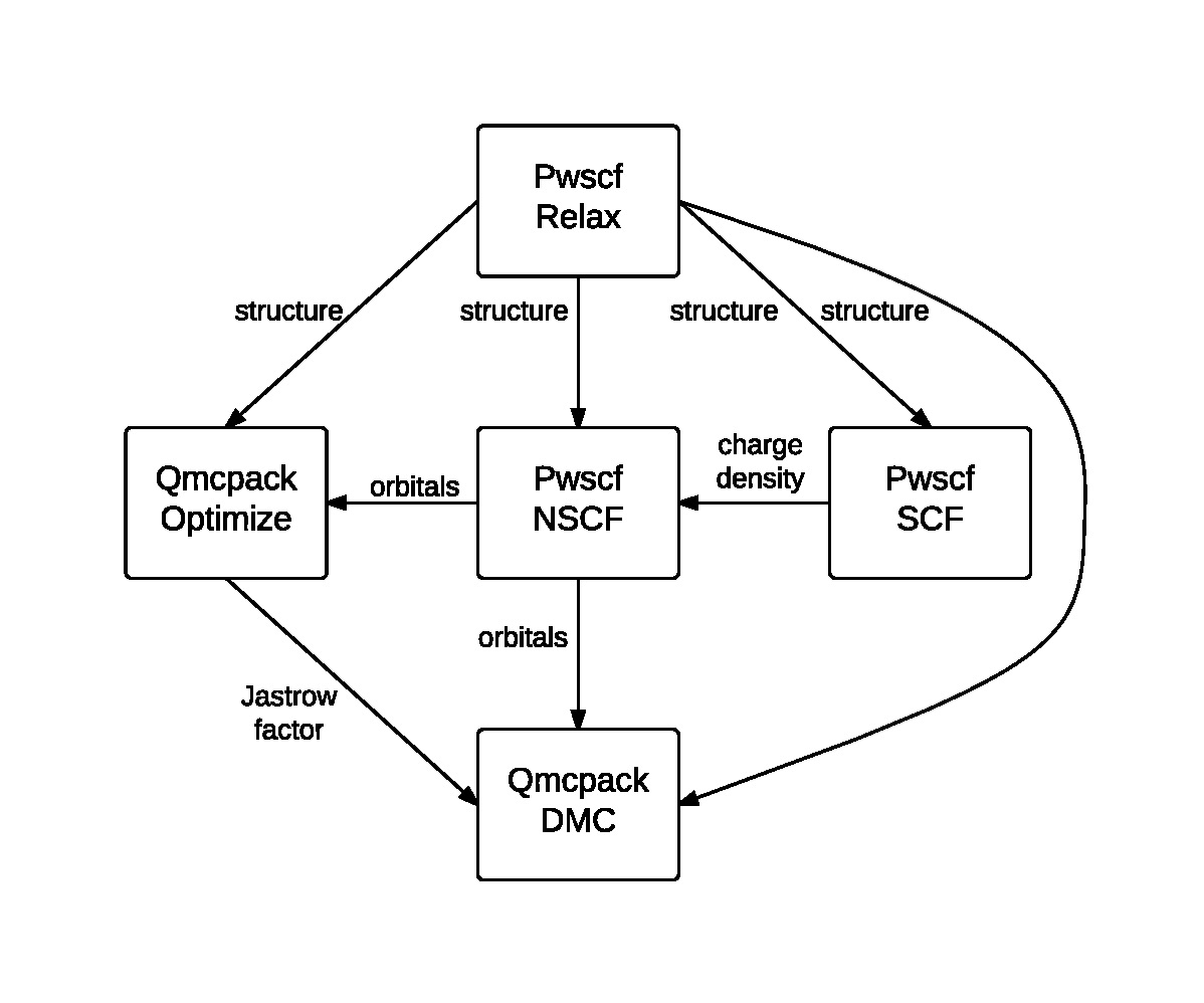
Fig. 1 An example Nexus workflow/cascade involving QMCPACK and PWSCF. The arrows and labels denote the flow of information between the simulation runs.

Composing workflows from simulation objects

Simulation workflows are created by specifying the data dependencies between simulation runs. An example workflow is shown in Fig. 1. In this case, a single relaxation calculation performed with PWSCF is providing a relaxed structure to each of the subsequent simulations. PWSCF is used to create a converged charge density (SCF) and then orbitals at specific k-points (NSCF). These orbitals are used by each of the two QMCPACK runs; the first optimization run provides a Jastrow factor to the final DMC run.

Below is an example of how this workflow can be created with Nexus. Most keywords to the generate functions have been omitted for brevity. The conv step listed below is implicit in Fig. 1.

relax = generate_pwscf(
    ...
    )

scf = generate_pwscf(
    dependencies = (relax,'structure'),
    ...
    )

nscf = generate_pwscf(
    dependencies = [(relax,'structure'     ),
                    (scf  ,'charge_density')],
    ...
    )

conv = generate_pw2qmcpack(
    dependencies = (nscf ,'orbitals' ),
    ...
    )

opt = generate_qmcpack(
    dependencies = [(relax,'structure'),
                    (conv ,'orbitals' )],
    ...
    )

dmc = generate_qmcpack(
    dependencies = [(relax,'structure'),
                    (conv ,'orbitals' ),
                    (opt  ,'jastrow'  )],
    ...
    )

As suggested at the beginning of this section, workflow composition logically breaks into two parts: simulation generation and workflow dependency specification. This type of breakup can also be performed explicitly within a Nexus user script, if desired:

# simulation generation
relax = generate_pwscf(...)
scf   = generate_pwscf(...)
nscf  = generate_pwscf(...)
conv  = generate_pw2qmcpack(...)
opt   = generate_qmcpack(...)
dmc   = generate_qmcpack(...)

# workflow dependency specification
scf.depends(relax,'structure')
nscf.depends((relax,'structure'     ),
             (scf  ,'charge_density'))
conv.depends(nscf ,'orbitals' )
opt.depends((relax,'structure'),
            (conv ,'orbitals' ))
dmc.depends((relax,'structure'),
            (conv ,'orbitals' ),
            (opt  ,'jastrow'  ))

More complicated workflows or scans over parameters of interest can be created with for loops and if-else logic constructs. This is fairly straightforward to accomplish because any keyword input can given a Python variable instead of a constant, as is mostly the case in the brief examples above.

Workflow execution

Simulation jobs are actually executed when the corresponding simulation objects are passed to the run_project function. Within the run_project function, most of the workflow management operations unique to Nexus are actually performed. The details of the management process is not the purpose of this section. This process is discussed in context in the Complete Examples walkthroughs.

The run_project function can be invoked in a couple of ways. The most straightforward is simply to provide all simulation objects directly as arguments to this function:

run_project(relax,scf,nscf,opt,dmc)

When complex workflows are being created (e.g. when the generate function appear in for loops and if statements), it is generally more convenient to accumulate a list of simulation objects and then pass the list to run_project as follows:

sims = []

relax = generate_pwscf(...)
sims.append(relax)

scf   = generate_pwscf(...)
sims.append(scf)

nscf  = generate_pwscf(...)
sims.append(nscf)

conv  = generate_pw2qmcpack(...)
sims.append(conv)

opt   = generate_qmcpack(...)
sims.append(opt)

dmc   = generate_qmcpack(...)
sims.append(dmc)

run_project(sims)

When the run_project function returns, all simulation runs should be finished.

Limiting the number of submitted jobs

Nexus will submit all eligible jobs at the same time unless told otherwise. This can be a large number when many calculations are present within the same project, e.g. various geometries or twists. While this is fine on local resources, it might break the rules at computing centers such as ALCF where only 20 jobs can be submitted at the same time. In such cases, it is possible to specify the size of the queue in Nexus to avoid monopolizing the resources.

from nexus import get_machine
theta = get_machine('theta')
theta.queue_size = 10

In this case, Nexus will never submit more than 10 jobs at a time, even if more jobs are ready to be submitted, or resources on the local machine are available. Having the option of limiting the number of jobs running at the same time can be useful even on local workstations (to avoid taking over all the available resources). In such a case, a simpler strategy is possible by claiming fewer available cores in settings, e.g. machine=’ws8’ vs ‘ws4’ vs ‘ws2’ etc.

Job bundling

Job bundling refers to aggregating multiple independent tasks into a single job submission to reduce queueing overhead and improve resource utilization. This approach is especially beneficial on systems that impose strict limits on the number of job submissions or priortize capability jobs over numberous small jobs.

The following provides an example of job bundling applied to the equation of state calculation for diamond:

from nexus import bundle

# Equilibrium lattice constant of diamond (Angstrom)
a_eqm = 3.57

bscfsims=[]

# Calculate diamond equation of state (energy vs. lattice constant)
for scale in [.80,.90,1.00,1.10,1.20]:

    a = scale*a_eqm

    # Details of the physical system
    system = generate_physical_system(
        units = 'A',                  # Angstrom units
        axes  = [[a/2, a/2,   0],     # Cell axes
                 [  0, a/2, a/2],
                 [a/2,   0, a/2]],
        elem  = ['C','C'],            # Element names
        posu  = [[0.00, 0.00, 0.00],  # Element positions (crystal units)
                 [0.25, 0.25, 0.25]],
        C     = 4,                    # Pseudpotential valence charge
        )

    # PBE calculation with Quantum ESPRESSO
    scf = generate_pwscf(
        identifier   = 'scf',                      # In/out file prefix
        path         = 'a_{:6.4f}'.format(a),      # Run directory
        job          = job(nodes=4,app='pw.x'),    # Job details
        input_type   = 'generic',                  # QE inputs below
        calculation  = 'scf',                      # SCF calculation
        input_dft    = 'pbe',                      # PBE functional
        ecutwfc      = 200,                        # PW energy cutoff (Ry)
        conv_thr     = 1e-8,                       # SCF conv threshold (Ry)
        system       = system,                     # System from above
        pseudos      = ['C.BFD.upf'],              # Pseudopotential files
        kgrid        = (4,4,4),                    # M.P. k-point grid
        kshift       = (0,0,0),                    # M.P. grid shift
        )

    bscfsims.append(scf)

#end for

# Job bundling
bsim = bundle(bscfsims)

# Execute the workflow
run_project()

Without job bundling, the example above results in 5 different job submissions, each using 4 nodes and corresponding to a different lattice constant of diamond. Since these jobs are mutually independent, they can be combined into a single 20 nodes (4 nodes * 5 tasks) job using bundle function as seen in the example. The bundled jobs can involve any combination of node counts and types of simulation. However, the simulations should have close to the same runtime to make the most efficient use of resources. The bundled jobs are not required to be combined into a single job. Their size can be adjusted by distributing tasks across separate bundle functions.

Customizing job options

The commands used to launch run jobs can be customized from those specified by the default machine definitions. Uses include customizing the options passed to MPI and customizing settings based on details of the runs.

For example, we can modify the MPI thread binding as follows:

settings(
  pseudo_dir = './pseudopotentials',
  results    = '',
  sleep      = 3,
  machine    = 'ws16',
  )

...

scf = generate_pwscf(
  job = job(cores=16,app='pw.x',run_options=dict(bind_to='--bind-to none')),
  ...
  )

which will result in output

Executing:
export OMP_NUM_THREADS=1
mpirun --bind-to none -np 16 pw.x -input scf.in

The options passed to the executable can also be modified. For example, to give different parallelization settings.

The following gives an example of modifying both the run and application options based on the machine the workflow is executing on:

settings(
  pseudo_dir = './pseudopotentials',
  results    = '',
  sleep      = 3,
  machine    = 'ws128',
  )

if settings.machine=='ws128':
    # jobs for 128 core workstation
    scf_opts1 = obj(app         = 'pw.x',
                    run_options = '--bind-to none')
    scf_opts2 = obj(app         = 'pw.x',
                    run_options = '--bind-to none',
                    app_options = '-nk 8')
    scf_job1 = job(cores= 64,**scf_opts1)
    scf_job2 = job(cores= 64,**scf_opts2)
    scf_job3 = job(cores=128,**scf_opts2)

elif settings.machine=='inti':
    # jobs for "Inti" cluster
    qe_presub = '''
module purge
module load mpi/openmpi-x86_64
module load qe/quantum-espresso
'''
    scf_opts1 = obj(nodes       = 1,
                    hours       = 1,
                    app         = 'pw.x',
                    run_options = '--bind-to none',
                    presub      = qe_presub)
    scf_opts2 = obj(nodes       = 1,
                    hours       = 1,
                    app         = 'pw.x',
                    run_options = '--bind-to none',
                    app_options = '-nk 8',
                    presub      = qe_presub)
    scf_job1 = job(processes_per_node=64,**scf_opts1)
    scf_job2 = job(processes_per_node=64,**scf_opts2)
    scf_job3 = job(**scf_opts2)

else:
    print('machine unknown!')
    exit()
#end if

Data analysis

Following the call to run_project, the user can perform data analysis tasks, if desired, as the analyzer object associated with each simulation contains a collection of post-processed output data rendered in numeric form (ints, floats, numpy arrays) and stored in a structured format. An interactive example for QMCPACK data analysis is shown below. Note that all analysis objects are interactively browsable in a similar manner.

>>> qa=dmc.load_analyzer_image()

>>> qa.qmc
  0                     VmcAnalyzer
  1                     DmcAnalyzer
  2                     DmcAnalyzer

>>> qa.qmc[2]
  dmc                   DmcDatAnalyzer
  info                  QAinformation
  scalars               ScalarsDatAnalyzer
  scalars_hdf           ScalarsHDFAnalyzer

>>> qa.qmc[2].scalars_hdf
  Coulomb               obj
  ElecElec              obj
  Kinetic               obj
  LocalEnergy           obj
  LocalEnergy_sq        obj
  LocalPotential        obj
  data                  QAHDFdata

>>> print qa.qmc[2].scalars_hdf.LocalEnergy
  error           = 0.0201256357883
  kappa           = 12.5422841447
  mean            = -75.0484800012
  sample_variance = 0.00645881103012
  variance        = 0.850521272106

Twist averaged calculations

This section describes several special features and capabilities to make specifying and running of twist-averaged calculations more convenient and efficient.

Twist occupation specification

Gapped systems

For QMC calculations involving twist-averaging, Nexus can set the desired twist occupations for the spin up and down electron channels. By default, the spin up and down occupations for each twist will be equal (non-magnetic phase) and each twist will be charge neutral. If a ferromagnetic type phase is required in gapped systems, net_spin argument can be specified in the generate_physical_system() function. This will result in each twist having magnetization equal to net_spin while still preserving charge neutrality in each twist. Specifying net_spin is sufficient for gapped systems since the charge and the net spin should not vary from twist to twist.

Metallic systems

The charge and the net spin are expected to vary from twist to twist in metallic systems in general. In Nexus, this can be handled via grand-canonical twist-averaging (GCTA), by specifying the gcta argument in the generate_qmcpack() function. The gcta argument can take the values given in Table 2. Currently, only workflows that use Quantum ESPRESSO (PWSCF) are supported by gcta.

Table 2 Available GCTA flavors in Nexus and their descriptions. The “charge-neutrality” indicates if the GCTA flavor guarantees \(\sum_{i}^{N} q_i = 0\) where \(i\) is the twist index.

gcta	charge-neutrality	k-point symmetry	spinors	description
'nscf'	No	Supported	Supported	NSCF Fermi level
'scf'	No	Supported	Supported	SCF Fermi level
'afl'	Yes	Not supported	Supported	Adapted Fermi level
'safl'	Yes	Not supported	Not supported	Spin-adapted Fermi level

Additional information:

• 'nscf': Use the non-self-consistent-filed (NSCF) Fermi level to determine the twist occupations. Nexus will attempt to traceback one level in PWSCF dependencies to read the NSCF Fermi level from the pwscf_output/pwscf.xml file.

• 'scf': Use the self-consistent-filed (SCF) Fermi level to determine the twist occupations. Nexus will attempt to traceback two levels in PWSCF dependencies to read the SCF Fermi level from the pwscf_output/pwscf.xml file. Due to this, the NSCF simulation should be in a separate path from the SCF simulation to avoid overwriting.

• 'afl': Use an adapted Fermi level determined from the available sorted eigenvalues that will give a net charge-neutral system [AGK24]. The Fermi level is determined solely from the eigenvalues in pwscf.pwscf.h5. Therefore, Nexus will not attempt to traceback anything in dependencies in this case.

• 'safl': Use a spin-adapted Fermi level determined by sorting each spin channel separately and using the SCF magnetization as target magnetization, while achieving net charge-neutrality [AGK24]. Since it requires the SCF magnetization, Nexus will attempt to traceback two levels in PWSCF dependencies to read the total magnetization from the pwscf_output/pwscf.xml file. Due to this, the NSCF simulation should be in a separate path from the SCF simulation to avoid overwriting.

Caution:

• Note that the net_spin will be overwritten by the gcta for the specified QMC simulation object. This is because the net magnetization of the system is now defined by the Fermi level. For example, in 'afl', the net magnetization is uniquely determined by the single-particle eigenvalues. In 'safl', the net magnetization is chosen as close as possible to the SCF magnetization.

• Note that gcta flavors 'scf' and 'nscf' do not guarantee a net charge-neutrality. They were implemented for comparison and research purposes only. Therefore, these are not likely to be useful in production runs.

Current limitations:

• The 'afl' and 'safl' options require a twist-averaging without k-point symmetry, i.e., using the full k-points with equal weights instead of the reduced k-points with varying weights. The reason is that the existence of weights in k-points can prevent determining a Fermi level that will result in a charge-neutral system. Effectively, it requires fractional charges in twists, which is not nominally possible in QMCPACK. However, it could be possible to achieve net charge-neutrality by adding extra k-points with certain required charges. This is currently not implemented.

• Currently, the twist occupations are calculated by first determining the Fermi level requested by gcta flavor and then occupying all single-particle eigenvalues below this energy (\(e_i < E_F\)). Some initial uses of gcta showed issues with eigenvalue degeneracies near the Fermi level, leading to a net non-zero charge. In most cases, this is not an issue due to the residual convergence error in NSCF, which effectively acts as a small randomizer of eigenvalues. However, it is possible to avoid this issue altogether, which requires re-implementation of gcta. In this new potential version, a table of sorted eigenvalues and the k-points they folded from are kept together. Then, since the number of electrons that needs to be occupied is known, the occupations can be set for each k-point and their folded twists. It avoids the (\(e_i < E_F\)) comparison which is numerically problematic if there are eigenvalue degeneracies.

• Due to the hard-coded nature of the limited dependency traceback capability implemented in gcta, hybrid functionals in PWSCF will currently not work with safl and scf. This is because NSCF calculations are not possible with the hybrid functionals, requiring a direct (scf -> pw2qmcpack) instead of (scf -> nscf -> pw2qmcpack).

• gcta argument will currently not work if there is a single twist in the system (it only activates when there are multiple twists).

• gcta currently supports only Quantum ESPRESSO (PWSCF).

Please contact the developers if any of these issues are critical for research.

Bundling of twist-averaged jobs

Twist averaged calculations will be run as a single job and QMCPACK invocation by default, dividing the total requested number of nodes & tasks by the total number of twists. This requires and will only work if the number of twists perfectly divides into the requested computational resources. For example, a job requesting 8 nodes with 4 total twists would use 2 nodes per twist, while a job with 5 twists would need to request a multiple of 5 nodes by default. Depending on details of the machine, it may be preferable to run the individual twist calculations separately or to automatically scale the size of the job according to the number of twists.

The twists can be run as individual jobs using the following:

ntwists = len(system.structure.kpoints)
qmc_job = job(processes=1,threads=2,hours=8)
for n in range(ntwists):
    qmc = generate_qmcpack(id       = 'dmc.g'+str(n).zfill(3),
                           twistnum = n,
                           job      = qmc_job,
                           ...)

Note that when the above approach is used, the twist_info.dat files are not currently created. When analysing the results, care should be taken to apply the correct weight to each twist.

A job can be scaled proportionally to the number of twists as follows:

system = generate_physical_system(...)
N = 10
M = len(system.structure.kpoints)
qmc_job = job(nodes=N*M,...)
qmc = generate_qmpcack(job=qmc_job,...)

Nexus command line options

Nexus user scripts process a number of command line options. These override settings in the script. They are most commonly used to check the status of workflows (--status_only) and to check the generated workflows during development (--generate_only).

• --status_only : Report status of all simulations and then exit.

• --status : Controls displayed simulation status information. May be set to one of ‘standard’, ‘active’, ‘failed’, or ‘ready’.

• --generate_only : Write inputs to all simulations and then exit. Note that no dependencies are processed, e.g., if one simulation depends on another for an orbital file location or for a relaxed structure, this information will not be present in the generated input file for that simulation since no simulations are actually run with this option.

• --graph_sims : Display a graph of simulation workflows, then exit.

• --progress_tty : Print abbreviated polling messages. The polling message normally written to a newline every polling period will instead be overwritten in place, greatly shortening the output.

• --sleep : Number of seconds between polls. At each poll, new simulations are run once all simulations they depend on have successfully completed. A status line is printed every poll.

• --machine : Name of the machine the simulations will be run on. Workstations with between 1 and 128 cores may be specified by ‘ws1’ to ‘ws128’ (works for any machine where only mpirun is used).

• --account : Account name required to submit jobs at some HPC centers.

• --runs : Directory name to perform all runs in. Simulation paths are appended to this directory.

• --results : Directory to copy out lightweight results data. If set to ‘’, results will not be stored outside of the runs directory.

• --local_directory : Base path where runs and results directories will be created

• --pseudo_dir : Path to directory containing pseudopotential files.

• --basis_dir : Path to directory containing basis set files (useful if running Gaussian-basis based QMC workflows).’

• --ericfmt : Path to the ericfmt file used with GAMESS (required by GAMESS).

• --mcppath : Path to the mcpdata file used with GAMESS (optional for most workflows).

• --vdw_table : Path to the vdw_table file used with Quantum ESPRESSO (required only if running Quantum ESPRESSO with van der Waals functionals).

• --qprc : Path to the quantum_package.rc file used with Quantum Package.

[AGK24] (1,2)

Abdulgani Annaberdiyev, Panchapakesan Ganesh, and Jaron T. Krogel. Enhanced Twist-Averaging Technique for Magnetic Metals: Applications Using Quantum Monte Carlo. Journal of Chemical Theory and Computation, 2024. doi:10.1021/acs.jctc.4c00058.